blog 4 (DOE)
Hi everyone! 😀 Welcome back to my blog where I’d be sharing about my experience applying DOE in a practical setting as well as a case study! Without further ado, let’s get into it.
Design of experiments (DOE) is the backbone for any product design as well as product improvement efforts. It is a methodology to obtain knowledge of a complex, multivariable process with the fewest number of trials possible to educate the user on the relationships between each factor.
With that let us look at a case study where we can apply our concept of DOE.
CASE STUDY:
What could be simpler than making microwave popcorn? Unfortunately, as everyone who has ever made popcorn knows, it’s nearly impossible to get every kernel of corn to pop. Often a considerable number of inedible “bullets” (un-popped kernels) remain at the bottom of the bag. What causes this loss of popcorn yield?In this case study, three factors were identified:
1. Diameter of bowls to contain the corn, 10 cm and 15 cm
2. Microwaving time, 4 minutes and 6 minutes
3. Power setting of microwave, 75% and 100%
8 runs were performed with 100 grams of corn used in every experiments and the measured variable is the amount of “bullets” formed in grams and data collected are shown below:
Factor A= diameter
Factor B= microwaving time
Factor C= power
FULL FACTORIAL METHOD:
Using the data present in the table, the HIGHS and LOWS of each factor can be obtained, enabling the average to be determined as well. A graph is plotted using the average values to determine the significance of each factor. The significance can be determined by looking at the steepness of the gradients.
Bullets (g) VS FACTOR LEVEL GRAPH
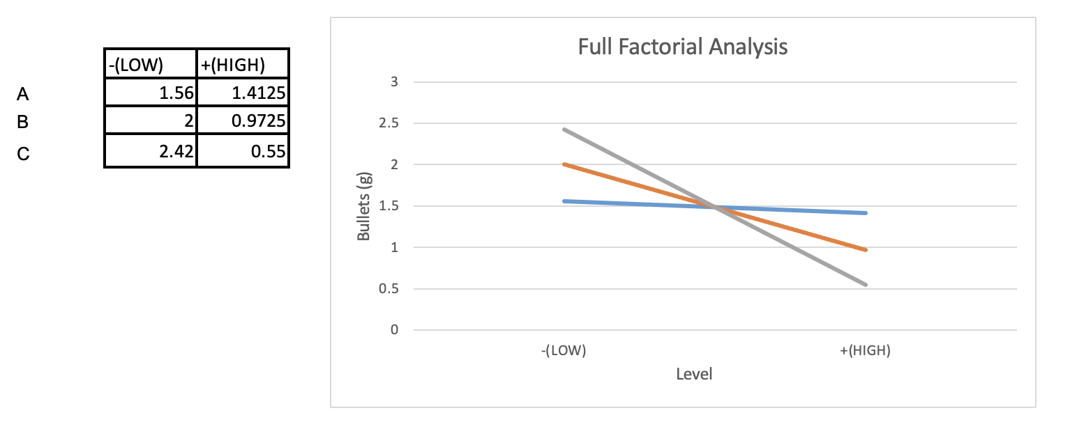
Legend:
Blue line = Factor A
Orange line = Factor B
Grey line = Factor C

EFFECTS OF SINGLE FACTORS AND THEIR RANKING:
As observed from the plot above, when the diameter increases from a LOW value of 10cm to a HIGH value of 15cm, the average mass of bullets decreases from 1.56g to 1.4125g. When the microwaving time increases from a LOW value of 4min to a HIGH value of 6min, the average mass of bullets decreases from 2g to 0.9725g. When the power setting increases from a LOW value of 75% to a HIGH value of 100%, the average mass of bullets decreases from 2.42g to 0.55g.
Factor C (power setting) has the greatest impact on the change in average mass of bullets when the level is changed from LOW to HIGH. Factor B has the second greatest impact on the change in average mass, while Factor A has the least impact. This can be seen from the graphs as the difference in average mass of bullets was the greatest for Factor C, hence indicating that it had the largest impact. Moreover, the gradient helps to identify the significance of the factors. Since Factor C had the steepest gradient, it had the greatest difference in average mass between the LOW and HIGH values.
INTERACTION EFFECTS OF FACTORS
Now that we’re familiar with the different factors, let us look at the interaction effects of the different factors. Two factors are said to interact with each other if the effect of one factor on the response variable is different at different levels of the other factor.
Interaction effects of AxB:
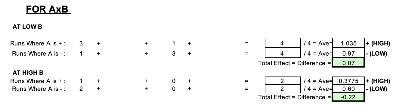

The gradients of both lines differ as the blue line (LOW B) has a positive gradient, while the orange line (HIGH B) has a negative gradient. Since the lines are non parallel, there is interaction present between A and B.
Interaction effects of BXC:
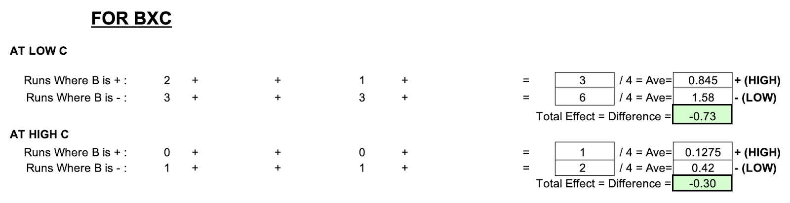

The gradients of both lines differ as the orange line (HIGH C) has a steeper gradient than the blue line (LOW C). Since the lines are non-parallel, there is a slight interaction present.
Interaction effects of AxC:
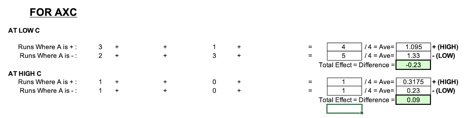
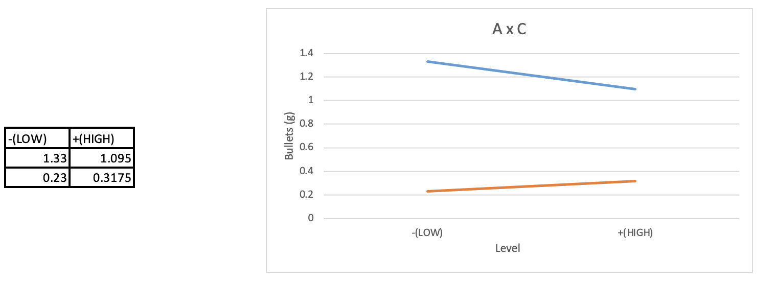
The gradients of both lines differ as the orange line (HIGH C) has a positive gradient while the blue line (LOW C) has a negative gradient. Since both lines are non-parallel, they have slight interaction present.
Conclusion:
In conclusion, Factor C had the greatest effect, followed by Factor B and lastly Factor A. Although interaction was present between all 3 factors, there was a difference in the significance of the interaction that could be determined by looking at the gradients of the plots above shown. Upon comparison, the interaction effects of AxB were the least, as compared to BxC and AxC.
FRACTIONAL FACTORIAL ANALYSIS:
To carry out Fractional factorial analysis, I will be using runs 1,2,3 and 6 since they have an equal number of HIGHS and LOWS for each factor during comparison. A graph is plotted using the average values to determine the significance of each factor. The significance can be determined by looking at the steepness of the gradients.


EFFECTS OF SINGLE FACTORS AND THEIR RANKINGS:
As observed from the fractional factorial plot above, when the diameter increases from a LOW value of 10cm to a HIGH value of 15cm, the average mass of bullets increases from 0.73g to 0.8775g. When the microwaving time increases from a LOW value of 4 min to a HIGH value of 6 min, the average mass of bullets decreases from 0.98g to 0.6275g. When the power setting increases from a LOW value of 75% to a HIGH value of 100%, the average mass of bullets decreases from 1.35g to 0.265g. Hence
Factor C (power setting) has the greatest impact on the change in average mass of bullets when the level is changed from LOW to HIGH. Factor B has the second greatest impact on the change in average mass, while Factor A has the least impact. This can be seen from the graphs as the difference in average mass of bullets was the greatest for Factor C, hence indicating that it had the largest impact. Moreover, the gradient helps to identify the significance of the factors. Since Factor C had the steepest gradient, it had the greatest difference in average mass between the LOW and HIGH values.
Conclusion:
In conclusion, Factor C had the greatest effect, followed by Factor B and lastly Factor A. However the graph plotted for fractional factorial analysis differs slightly from the graph plotted for full factorial analysis. This is because the gradient of A during full factorial analysis was positive but during fractional factorial analysis, the gradient of A was negative. Hence, this ultimately leads us to question the validity of the factors and the effects if we were to only use the available conditions.
LINK TO THE EXCEL SHEET (both full factorial and fractional factorial): https://drive.google.com/drive/folders/1P_gVaf09UWEH00A2EY5Ojb-puCHT_RyM
Learning reflection:
When I was first introduced to DOE, I did not realise its importance and significance in experiments and their role in improving experiments just yet. But after Mr Chua’s lesson on DOE, I became more aware of how DOE relates to chemical product design. DOE is known to be the backbone of any product design or product improvement efforts as it helps us determine the effects of different factors on the chemical product. Through analysing the interaction effects and the relationships of the factors, we would then be able to amend our chemical product to be of its best version.
Initially the biggest challenge I faced when I attempted to carry out DOE was plotting the graphs on EXCEL according to the data obtained. Although I’m generally competent in terms of using Microsoft softwares, I do struggle in terms of using EXCEL properly sometimes. Thankfully, Mr Chua was kind enough to demonstrate to the class on how to plot the EXCEL graphs for full factorial analysis and fractional factorial analysis! This made the entire plotting process easy and I even got to explore EXCEL and its different features. Hence I’m glad this practical not only taught me about DOE, but also encouraged me to improve on my technical skills such as EXCEL!
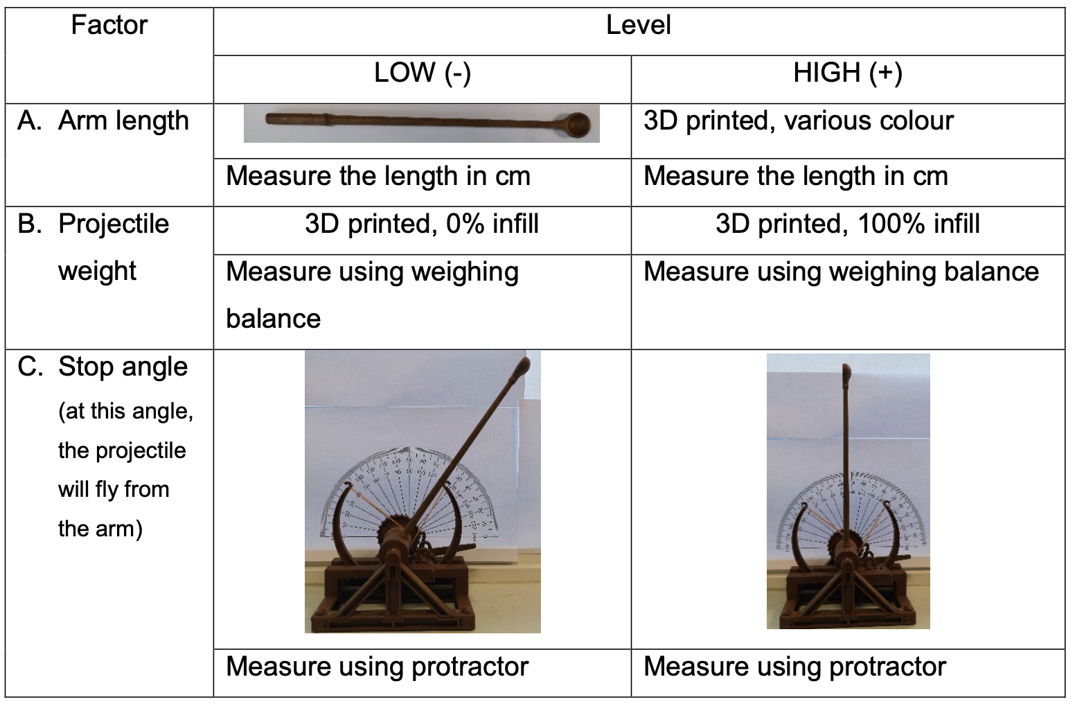
After we were more familiarised with the concept of DOE, we proceeded to apply this concept in a practical setting. During the practical, we were required to discover the significance of different factors (arm length, projectile weight and stop angle) on the distance travelled by the projectile. To tackle this task with efficiency, we divided our group into 2 smaller groups, where 1 group will be carrying out fractional factorial design analysis while the other group performed full factorial design analysis.
Factors vs Level:
After carrying out FULL FACTORIAL ANALYSIS, this was the data obtained:


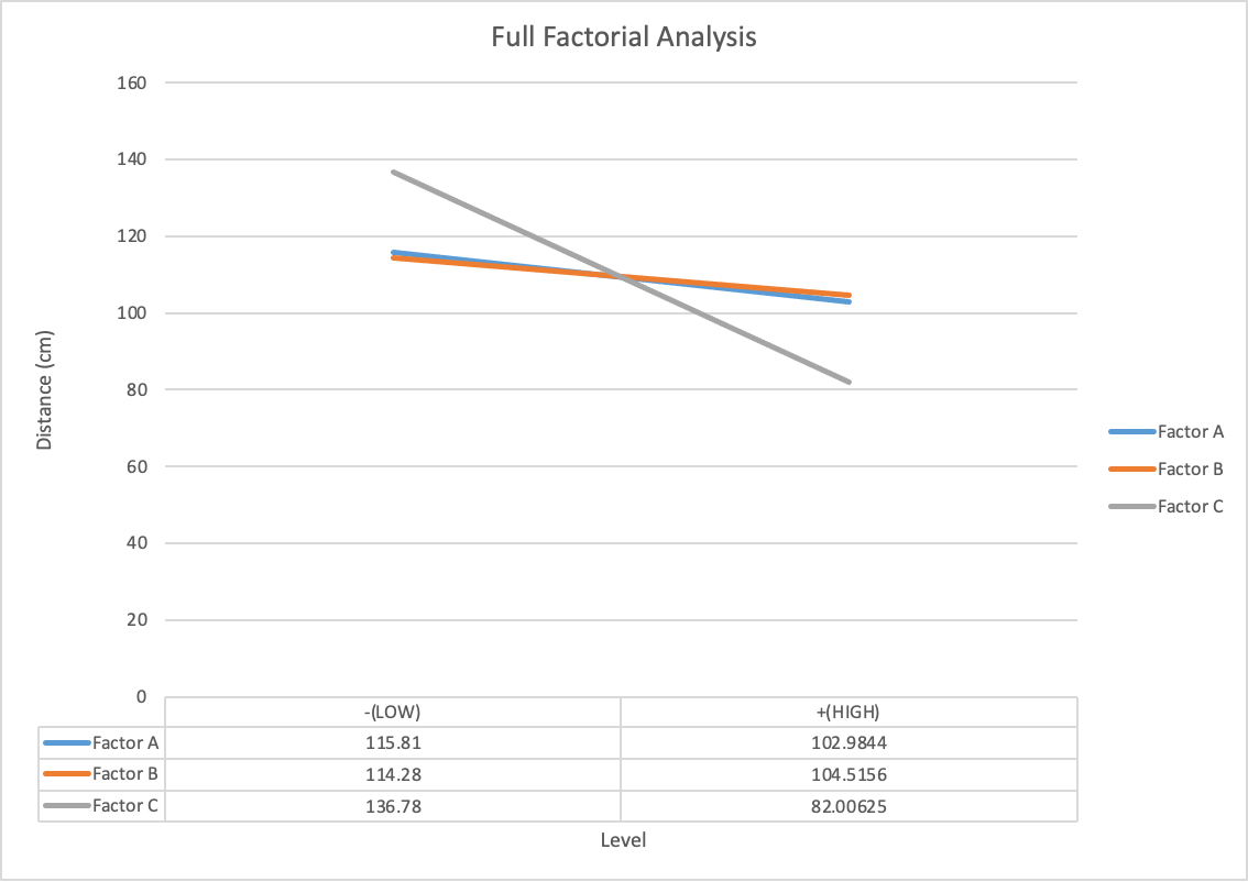
C (stop angle) is the most significant as when comparing the low value and the high value, you can see that there is a significant difference in distance travelled. When the high value is used the distance travelled can be up to 136 cm roughly while when using the low value the distance travelled can be reduced to as low as 82 cm roughly.
For factors B (projectile weight) and A (arm length), their impact on the distance travelled are very close. However, the arm length has a slightly higher impact when it comes to distance travelled as the difference between the low value and high value used has a slightly larger difference compared to projectile weight. Hence projectile weight is the least significant.
In summary, since C has the steepest gradient, it was the most significant factor, followed by A and lastly B.
After carrying out FRACTIONAL FACTORIAL ANALYSIS, this was the data obtained:

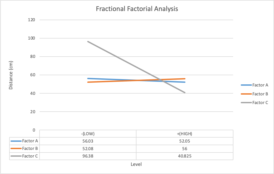
C (stop angle) is the most significant as when comparing the long value and the high value, you can see that there is a significant difference in distance travelled. When the high value is used the distance travelled can be up to 96 cm roughly while when using the low value the distance travelled can be reduced to as low as 40 cm roughly.
For factors B (projectile weight) and A (arm length), their impact on the distance travelled are very close. However, in the fractional factorial design, we can see that a lower value of A provides a more distance travelled, meaning that a shorter arm length would allow us to get more distance compared to a longer arm.
In summary, since Factor C has the steepest gradient, it has the largest significance, followed by Factor A with the second greatest significance. Factor B has the smallest significance as it has the smallest gradient.
After this activity, we participated in the group challenge where we needed to make use of the data we had already obtained, to knock down the 4 targets placed on the table. The catapult launcher was required to be placed behind a yellow line to ensure fairness to everyone. Since we were given 3 trial attempts for the challange, exclusing the actual 2 attempts for each target, we could perform some trial and error in order to knock the targets down. Although we did not manage to attain 1st place in this challenge, this was a great learning experience for my group as we had the opportunity to apply our learning in a practical situation.
Here are some videos from our practical session! 😋
Overall, this was a very engaging practical. I have now learnt the importance of DOE and its effect on creating the best version of a chemical product. I am excited to use this newly gained knowledge in my future endeavours and during my internship! 😇
Comments
Post a Comment